Contents

Example 4: LTI model of a Coleman tranformed wind turbine system

close all; clear; clc;

LTI model of a Coleman tranformed wind turbine system

% LTI system matrices
h = 0.1;             % Sample time
[OL,CL] = wtsLTI(h); % The wind turbine model
n = size(OL.a,1);    % The order of the system
r = size(OL.b,2);    % The number of inputs
l = size(OL.c,1);    % The number of outputs

Closed-loop identification experiment

Simulation of the model in closed loop

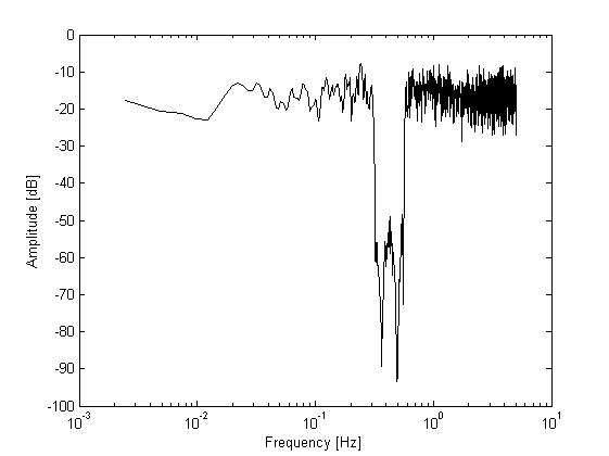
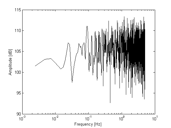
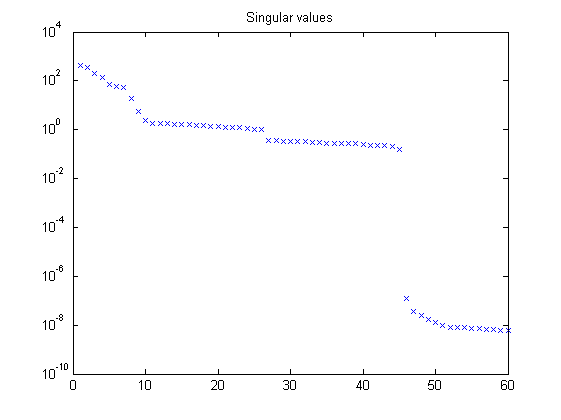
% Time sequence
N = 10000;  % number of data points
t = (0:h:h*(N-1))';

% Wind disturbance signals
d = randn(N,3);

% Excitation signal for pitch input
r_pitch = idprbs(N,1,h,5,0.4440,0,2);
ns = floor((length(r_pitch)-N)/2);
r_pitch = r_pitch(ns+1:N+ns,1);

% Plot PSD
[M,F] = pwelch(r_pitch,[],[],[],1/h);
figure, semilogx(F,mag2db(M),'k','LineWidth',1)
xlabel('Frequency [Hz]');
ylabel('Amplitude [dB]');

% Excitation signal for Torque input
r_torque = idprbs(N,1e3,h,5,inf,0,2);
ns = floor((length(r_torque)-N)/2);
r_torque = r_torque(ns+1:N+ns,2);

% Excitation signal for Torque input
[M,F] = pwelch(r_torque,[],[],[],1/h);
figure, semilogx(F,mag2db(M),'k','LineWidth',1)
xlabel('Frequency [Hz]');
ylabel('Amplitude [dB]');

% Add together for simulation
r = [r_pitch zeros(N,2) r_torque zeros(N,2)];

% Simulation of the closed-loop system
y = lsim(CL,[d r],t);

% Input and output selaction with scaling
ui = detrend(y(:,7:8),'constant');   % selects input for identification (excitation of pitch + control)
yi = detrend(y(:,1:3),'constant');   % selects output for identification
ri = [r_pitch r_torque];
[us,Du,ys,Dy] = sigscale(ui,yi); % signal scaling

% Closed-loop Spectral Analysis
[G,w] = spaavf(ui,yi,ri,h,10);
OLa = frd(G,w);

% Defining a number of constants
p = 50;     % past window size
f = 20;     % future window size

% PBSID-opt
[S,x] = dordvarx(us,ys,f,p,'tikh','gcv');
figure, semilogy(S,'x');
title('Singular values')
x = dmodx(x,n);
[Ai,Bi,Ci,Di,Ki] = dx2abcdk(x,us,ys,f,p);
%[Ai,Bi,Ci,Di,Ki] = dx2abcdk(x,us,ys,f,p,'stable'); % forces stability
Dat = iddata(ys',us',h);
Mi = abcdk2idss(Dat,Ai,Bi,Ci,Di,Ki);

% Variance-accounted-for (by Kalman filter)
yest = predict(Mi,Dat);
x0 = findstates(Mi,Dat);
disp('VAF of identified system')
vaf(ys,yest.y)

Warning: The frequency to be filtered out, Inf Hz, is larger than the
cutoff frequency 5 Hz 
Warning: >>> Skipping band stop filtering around Inf Hz <<< 
VAF of identified system

ans =

   99.9730
   98.4171
   99.9374

Prediction error method optimization

% Optimize identified system
set(Mi,'SSParameterization','Free','DisturbanceModel','Estimate','nk',zeros(1,2));
Mp = pem(Dat,Mi);

% Variance-accounted-for (by Kalman filter)
yest = predict(Mp,Dat);
x0 = findstates(Mp,Dat);
disp('VAF of optimized system')
vaf(ys,yest.y)

VAF of optimized system

ans =

   99.9739
   98.4633
   99.9454

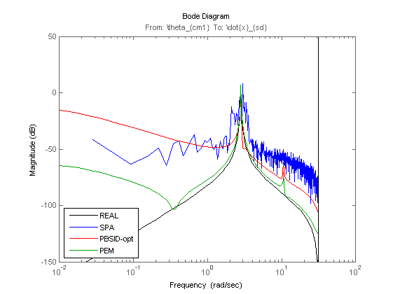
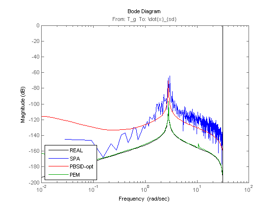
Identification results

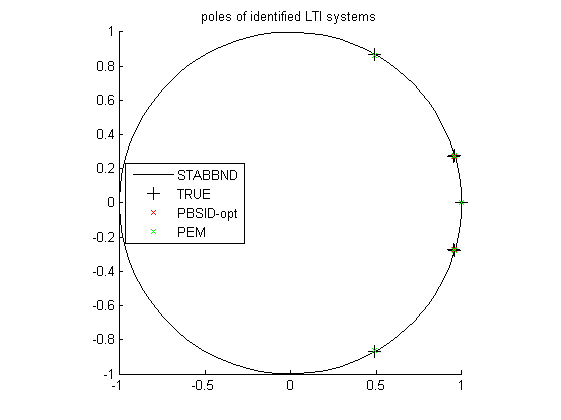
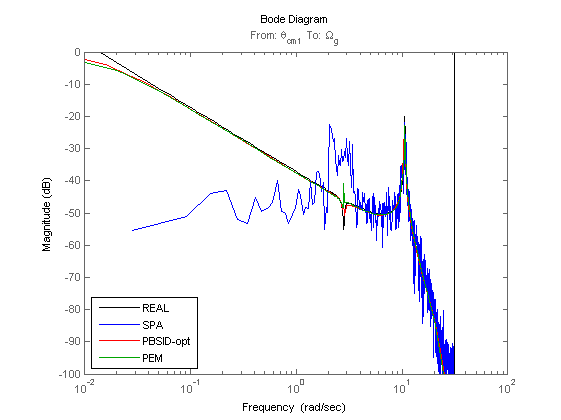
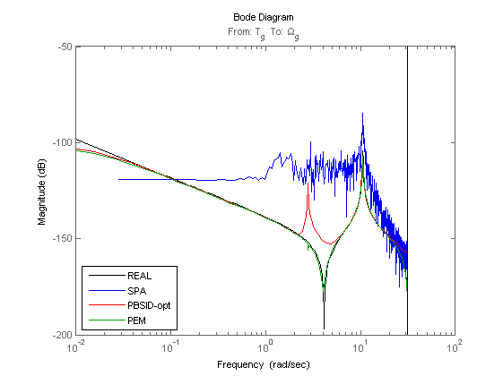
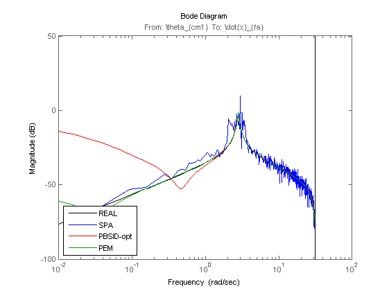
% Plot eigenvalues
figure
hold on
title('poles of identified LTI systems')
[cx,cy] = pol2cart(linspace(0,2*pi),ones(1,100));
plot(cx,cy,'k');
plot(real(eig(OL.a)),imag(eig(OL.a)),'k+','LineWidth',0.1,'MarkerEdgeColor','k', 'MarkerFaceColor','k', 'MarkerSize',10);
plot(real(eig(Mi.a)),imag(eig(Mi.a)),'rx');
plot(real(eig(Mp.a)),imag(eig(Mp.a)),'gx');
axis([-1 1 -1 1]);
axis square
legend('STABBND','TRUE','PBSID-opt','PEM','Location','West');
hold off

% Bodediagram (open loop)
OLi = ss(Mi);
OLp = ss(Mp);
OLi = Dy*OLi(1:3,1:2)*inv(Du);
OLp = Dy*OLp(1:3,1:2)*inv(Du);
figure, bodemag(OL(1,4),'k',OLa(1,1),'b',OLi(1,1),'r',OLp(1,1),'g');
axis([0.01 100 -100 0]);
legend('REAL','SPA','PBSID-opt','PEM','Location','SouthWest');
figure, bodemag(OL(1,7),'k',OLa(1,2),'b',OLi(1,2),'r',OLp(1,2),'g');
axis([0.01 100 -200 -50]);
legend('REAL','SPA','PBSID-opt','PEM','Location','SouthWest');
figure, bodemag(OL(2,4),'k',OLa(2,1),'b',OLi(2,1),'r',OLp(2,1),'g');
axis([0.01 100 -100 50]);
legend('REAL','SPA','PBSID-opt','PEM','Location','SouthWest');
figure, bodemag(OL(3,4),'k',OLa(3,1),'b',OLi(3,1),'r',OLp(3,1),'g');
axis([0.01 100 -150 50]);
legend('REAL','SPA','PBSID-opt','PEM','Location','SouthWest');
figure, bodemag(OL(3,7),'k',OLa(3,2),'b',OLi(3,2),'r',OLp(3,2),'g');
axis([0.01 100 -200 0]);
legend('REAL','SPA','PBSID-opt','PEM','Location','SouthWest');

Published with MATLAB® 7.9