Contents

Example 16: Fourth-order Hammerstein-Wiener model

close all; clear; clc;

The fourth-order LTI model with coloured process noise

% state-space matrices
A = [0.67 0.67 0 0; -0.67 0.67 0 0; 0 0 -0.67 -0.67; 0 0 0.67 -0.67];
B = [0.6598 -0.5256; 1.9698 0.4845; 4.3171 -0.4879; -2.6436 -0.3416];
K = [-0.6968 -0.1474; 0.1722 0.5646; 0.6484 -0.4660; -0.9400 0.1032];
C = [-0.3749 0.0751 -0.5225 0.5830; -0.8977 0.7543 0.1159 0.0982];
D = zeros(2);

% open-loop system
OL = ss(A,[B K],C,[D eye(2)],1);

Open-loop identification experiment

Simulation of the model in open loop

% input signals
N = 1000; % number of samples
t = (0:N-1)';   % time samples
r = randn(N,2); % excitation signal
fu = [sinc(r(:,1)).*r(:,1).^2 sin(r(:,2))];

% noise
e = 0.04.*randn(N,2); % noise signal

% simulation of open loop
y0 = lsim(OL,[fu zeros(N,2)],t);
y = lsim(OL,[fu e],t);
fy = [sign(y(:,1)).*sqrt(abs(y(:,1))) sign(y(:,2)).*sqrt(abs(y(:,2)))];
disp('Signal to noise ratio (SNR) (open-loop)')
snr(y,y0)

Signal to noise ratio (SNR) (open-loop)

ans =

   26.8787   24.1876

Identification of the model in open loop

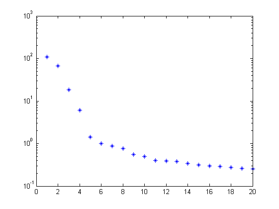
% parameters
n = 4;    % order of system
f = 10;   % future window size
p = 10;   % past window size

% PBSID-varx
[us,Du,ys,Dy] = sigscale(r,fy);
[S,x,fui,yi] = hwordvarx(us,ys,f,p,1e-4,1e-8);
figure, semilogy(S,'*');
x = hwmodx(x,n);
[Ai,Bi,Ci,Di,Ki] = hwx2abcdk(x,fui,yi,f,p);

Verification results

% variance accounted for (open loop)
Qu = fui*pinv(fu(p+1:p+size(fui,2),:)');
Qy = (Dy\y(p+1:p+size(yi,2),:)')*pinv(yi);
OLi = ss(Ai,(Bi*Qu)/Du,Dy*Qy*Ci,Dy*((Qy*Di*Qu)/Du),1);
yv = lsim(OL(1:2,1:2),fu,t);
ye = lsim(OLi,fu,t);
disp('VAF (open-loop)')
vaf(yv,ye)

VAF (open-loop)

ans =

   99.8561
   99.0690

Identification results

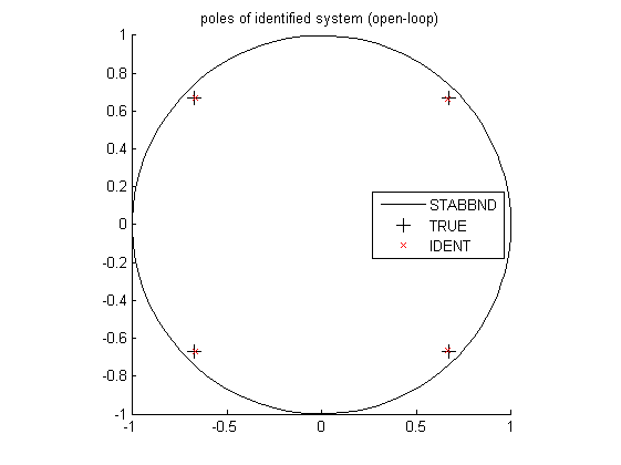
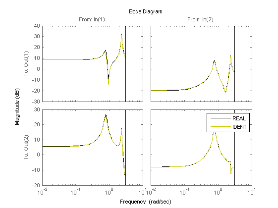
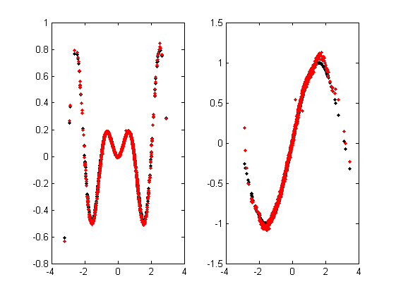
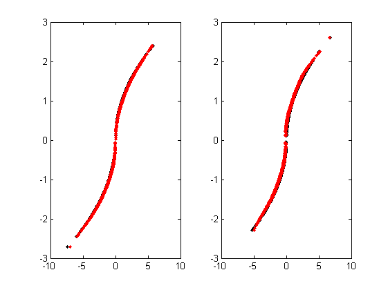
% plot eigenvalues (open loop)
figure
hold on
title('poles of identified system (open-loop)')
[cx,cy] = pol2cart(linspace(0,2*pi),ones(1,100));
plot(cx,cy,'k');
plot(real(pole(OL)),imag(pole(OL)),'k+','LineWidth',0.1,'MarkerEdgeColor','k','MarkerFaceColor','k','MarkerSize',10);
plot(real(eig(Ai)),imag(eig(Ai)),'rx');
axis([-1 1 -1 1]);
axis square
legend('STABBND','TRUE','IDENT','Location','East');
hold off

% simulation (open loop)
figure, bodemag(OL(1:2,1:2),'k',OLi,'y');
legend('REAL','IDENT');

% plot the non-linear function
fui = Qu\(Du*fui);
figure, subplot(1,2,1), plot(r(:,1),fu(:,1),'k.',r(p+1:p+size(fui,2),1),fui(1,:)','r.')
subplot(1,2,2), plot(r(:,2),fu(:,2),'k.',r(p+1:p+size(fui,2),2),fui(2,:)','r.')

% plot the non-linear function
yi = Dy*Qy*yi;
figure, subplot(1,2,1), plot(y(:,1),fy(:,1),'k.',yi(1,:)',fy(p+1:p+size(yi,2),1),'r.');
subplot(1,2,2), plot(y(:,2),fy(:,2),'k.',yi(2,:)',fy(p+1:p+size(yi,2),2),'r.');

Published with MATLAB® 7.9