Contents

Example 23: Periodic-LPV model of a wind turbine system

close all; clear; clc;

LPV model of a wind turbine system

% LPV system
h = 0.1;    % sample time
M = wtsLPV(h);
[l,r,n,m] = size(M);

Closed-loop identification experiment

Simulation of the model in closed loop

% Parameters
j = 35;     % period
np = 1000;  % number of periods
N = np*j;   % number of data points

% Measured data from the scheduling parameters
t = (0:h:h*(N-1))';
Omr = 2*pi/(h*j);
mu1 = sin(Omr*t);
mu2 = sin(Omr*t+2/3*pi);
mu3 = -mu1-mu2;
mu = [ones(N,1) mu1 mu2];

% Distarbance and excitation signals
u = [randn(N,3) randn(N,3) 1e3.*randn(N,1)];

% Simulation of the LPV system in closed loop
options = simset('solver','FixedStepDiscrete');
[t,x,y] = sim('SwtsLPV',[t(1) t(end)],options,[t u mu(:,2:3)]);
u = [y(:,7:9) u(:,7)];
y = y(:,1:6);

% signal scaling and trending
[us,Du,ys,Dy] = sigscale(u,y);

Identification of the model in closed loop

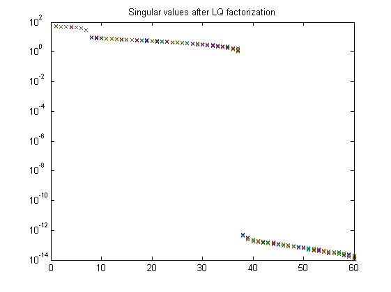
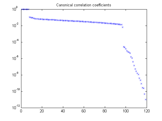
% Defining a number of constants
p = 12;     % past window size
f = 10;     % future window size

% Periodic-LPV identification
ckeep = [1 1 1 1 1 1;
       0 0 0 1 1 1;
       0 0 0 1 1 1]'; % do not keep the first three outputs of C1 and C2
pnd = pschedclust(mu,f,p);
[S,x,TU,K] = pordvarx(us,ys,mu,f,p,pnd,'none','gcv',0,[2 0 0 1 0],ckeep);
[x,CC] = pmodx(x,TU,K,n,[1e-12 1e-8 1e-6 1e-4],[1e-12 1e-8 1e-6 1e-4]);
[A,B,C,D,K] = px2abcdk(x,us,ys,mu,f,p,[2 0 0 1 0],pnd);

% Plot singular values and canonocal coefficients
figure, semilogy(S,'x');
title('Singular values after LQ factorization')
figure, semilogy(CC,'x');
title('Canonical correlation coefficients')

Optimize results with the prediction error method

Mid = idafflpv(A,B,C,D,K,[],h);
% [Mp,us,ys] = idafflpvA2idss(Mid,us,ys,mu(:,2:3));
% set(Mp,'SSParameterization','Free','DisturbanceModel','Estimate','nk',zeros(1,size(D,2)));
% Mp = pem(iddata(ys,us,h),Mp);
% Mp = idss2idafflpvA(Mp,m);

Verification results

% Simulation of real LPV system
uv = [zeros(N,3) randn(N,3) 1e3.*randn(N,1)];
yv = sim(M,uv,t,[mu1 mu2 mu3]);

% Simulation of identified LPV system
Mid.b = B*(kron(eye(m),inv(Du)));
Mid.c = Dy*C;
Mid.d = Dy*D*(kron(eye(m),inv(Du)));
yid = sim(Mid,uv(:,4:end),t,mu(:,2:3));
disp('VAF of identified LPV system')
vaf(yv,yid)

VAF of identified LPV system

ans =

   97.9819
   99.7006
   99.5031
   98.3372
   99.8716
   99.2135

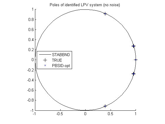
Identification results

% Plot eigenvalues
figure
hold on
title('Poles of identified LPV system (no noise)')
[cx,cy] = pol2cart(linspace(0,2*pi),ones(1,100));
plot(cx,cy,'k');
Ad = M.a;
plot(real(eig(Ad(:,1:n))),imag(eig(Ad(:,1:n))),'k+','LineWidth',0.1,'MarkerEdgeColor','k', 'MarkerFaceColor','k', 'MarkerSize',10);
plot(real(eig(A(:,1:n))),imag(eig(A(:,1:n))),'bx');
axis([-1 1 -1 1]);
legend('STABBND','TRUE','PBSID-opt','Location','West');
axis square
hold off

Published with MATLAB® 7.9