Contents

Example 2: Fourth-order LTI model without process noise in closed loop

close all; clear; clc;

The fourth-order LTI model without process noise

% state-space matrices
A = [0.67 0.67 0 0; -0.67 0.67 0 0; 0 0 -0.67 -0.67; 0 0 0.67 -0.67];
B = [0.6598 -0.5256; 1.9698 0.4845; 4.3171 -0.4879; -2.6436 -0.3416];
C = [-0.3749 0.0751 -0.5225 0.5830; -0.8977 0.7543 0.1159 0.0982];
D = zeros(2);

% open-loop system
OL = ss(A,B,C,D,1);

% closed-loop system
F = diag([0.25 0.25]);
CL = feedback(OL,F,[1 2],[1 2],-1);

Open-loop identification experiment

Simulation of the model in open loop

% input signals
N = 4000; % number of samples
t = (0:N-1)';   % time samples
r = randn(N,2); % excitation signal

% noise
e = randn(N,2); % noise signal

% simulation
y0 = lsim(OL,r,t);
y = y0 + e;
disp('Signal to noise ratio (SNR) (open-loop)')
snr(y,y0)

Signal to noise ratio (SNR) (open-loop)

ans =

   19.9194   15.9825

Identification of the model in open loop

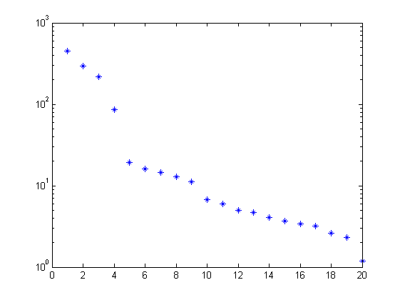
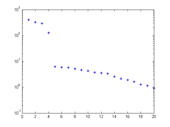
% parameters
n = 4;    % order of system
f = 10;   % future window size
p = 20;   % past window size

% PBSID-fir
[S,X] = dordfir(r,y,f,p,'tikh','gcv');
figure, semilogy(S,'*');
x = dmodx(X,n);
[Ai,Bi,Ci,Di] = dx2abcd(x,r,y,f,p);

% PBSID-varx
[S,X] = dordvarx(r,y,f,p,'tikh','gcv');
figure, semilogy(S,'*');
x = dmodx(X,n);
[Av,Bv,Cv,Dv,Kv] = dx2abcdk(x,r,y,f,p);

Verification results

% verification using variance accounted for (VAF) (open loop)
OLi = ss(Ai,Bi,Ci,Di,1);
OLv = ss(Av,Bv,Cv,Dv,1);
y = lsim(OL,r,t);
yi = lsim(OLi,r,t);
yv = lsim(OLv,r,t);
disp('VAF with PBSIDopt-fir (open loop)')
vaf(y,yi)
disp('VAF with PBSIDopt-varx (open-loop)')
vaf(y,yv)

VAF with PBSIDopt-fir (open loop)

ans =

   96.8178
   96.7164

VAF with PBSIDopt-varx (open-loop)

ans =

   99.9618
   99.9463

Identification results

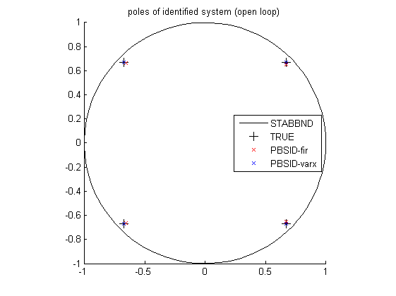
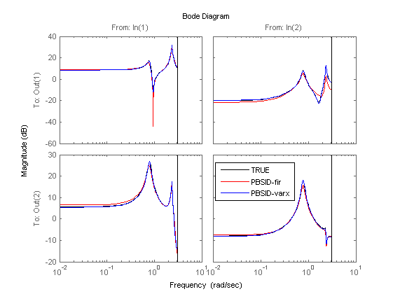
% plot eigenvalues (open loop)
figure
hold on
title('poles of identified system (open loop)')
[cx,cy] = pol2cart(linspace(0,2*pi),ones(1,100));
plot(cx,cy,'k');
plot(real(pole(OL)),imag(pole(OL)),'k+','LineWidth',0.1,'MarkerEdgeColor','k','MarkerFaceColor','k','MarkerSize',10);
plot(real(eig(Ai)),imag(eig(Ai)),'rx');
plot(real(eig(Av)),imag(eig(Av)),'bx');
axis([-1 1 -1 1]);
axis square
legend('STABBND','TRUE','PBSID-fir','PBSID-varx','Location','East');
hold off

% simulation
figure, bodemag(OL(1:2,1:2),'k',OLi,'r',OLv,'b');
legend('TRUE','PBSID-fir','PBSID-varx','Location','Best');

Closed-loop identification experiment

Simulation of the model in closed loop

% simulation of closed loop
y = lsim(CL,r,t) + 0.5.*e;
u = (r' - F*y')';
y0 = lsim(OL,u,t);
disp('Signal to noise ratio (SNR) (closed-loop)')
snr(y,y0)

Signal to noise ratio (SNR) (closed-loop)

ans =

   12.5731   15.3085

Identification of the model in closed loop

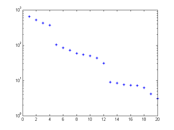
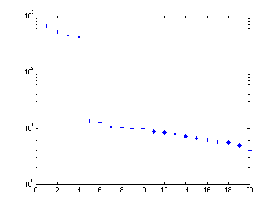
% PBSID-fir
[S,X] = dordfir(u,y,f,p,'tikh','gcv');
figure, semilogy(S,'*');
x = dmodx(X,n);
[Ai,Bi,Ci,Di] = dx2abcd(x,u,y,f,p);

% PBSID-varx
[S,X] = dordvarx(u,y,f,p,'tikh','gcv');
figure, semilogy(S,'*');
x = dmodx(X,n);
[Av,Bv,Cv,Dv,Kv] = dx2abcdk(x,u,y,f,p);

Verification results

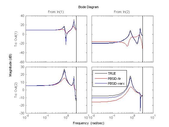
% verification using variance accounted for (VAF) (closed loop)
OLi = ss(Ai,Bi,Ci,Di,1);
OLv = ss(Av,Bv,Cv,Dv,1);
y = lsim(OL(1:2,1:2),u,t);
yi = lsim(OLi,u,t);
yv = lsim(OLv,u,t);
disp('VAF with PBSID-fir (closed-loop)')
vaf(y,yi)
disp('VAF with PBSID-varx (closed-loop)')
vaf(y,yv)

VAF with PBSID-fir (closed-loop)

ans =

   90.5044
   94.6283

VAF with PBSID-varx (closed-loop)

ans =

   99.7741
   99.8118

Identification results

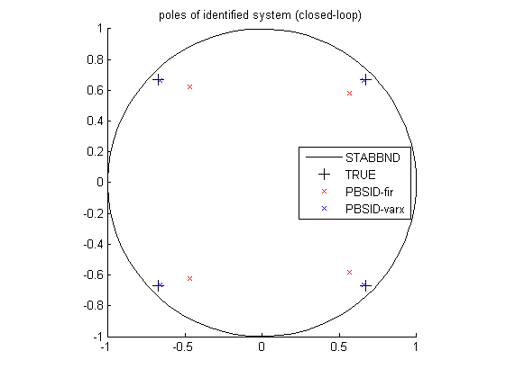
% plot eigenvalues (closed loop)
figure
hold on
title('poles of identified system (closed-loop)')
[cx,cy] = pol2cart(linspace(0,2*pi),ones(1,100));
plot(cx,cy,'k');
plot(real(pole(OL)),imag(pole(OL)),'k+','LineWidth',0.1,'MarkerEdgeColor','k','MarkerFaceColor','k','MarkerSize',10);
plot(real(eig(Ai)),imag(eig(Ai)),'rx');
plot(real(eig(Av)),imag(eig(Av)),'bx');
axis([-1 1 -1 1]);
axis square
legend('STABBND','TRUE','PBSID-fir','PBSID-varx','Location','East');
hold off

% simulation (closed loop)
figure, bodemag(OL(1:2,1:2),'k',OLi,'r',OLv,'b');
legend('TRUE','PBSID-fir','PBSID-varx','Location','Best');

Published with MATLAB® 7.9