Contents
Example 3: High-order LTI model of acoustical duct
close all; clear; clc;
The high-order LTI model (acoustical duct) with coloured process noise
% acoustical duct model
Ts = 0.001;
a = [1, -1.8937219532483e0, 9.2020408176247e-1, 8.4317527635809e-13,...
    -6.9870644340972e-13, 3.2703011891141e-13, -2.8053825784320e-14,...
    -4.8518619047975e-13, 9.0515016323085e-13, -8.9573340462955e-13,...
    6.2104932381850e-13, -4.0655443037130e-13, 3.8448359402553e-13,...
    -4.9321540807220e-13, 5.3571245452629e-13, -6.7043859898372e-13,...
    6.5050860651120e-13, 6.6499999999978e-1, -1.2593250989101e0,...
    6.1193571437226e-1];
b = [0, -5.6534330123106e-6, 5.6870704280702e-6, 7.7870811926239e-3,...
    1.3389477125431e-3, -9.1260667240191e-3, 1.4435759589218e-8,...
    -1.2021568096247e-8, -2.2746529807395e-9, 6.3067990166664e-9,...
    9.1305924779895e-10, -7.5200613526843e-9, 1.9549739577695e-9,...
    1.3891832078608e-8, -1.6372496840947e-8, 9.0003511972213e-3,...
    -1.9333235957678e-3, -7.0669966879457e-3, -3.7850561971775e-6,...
    3.7590122810601e-6];
c = [0, -5.65645330123106e-6, 5.345344280702e-6, 7.45341926239e-3,...
    2.3389477125431e-3, -9.5480667240191e-3, 1.545435759589218e-8,...
    -1.2343468096247e-8, -2.534549807395e-9, 4.454930166664e-9,...
    9.342424779895e-10, -7.2342313526843e-9, 1.9549739577695e-9,...
    1.564565078608e-8, -3.1272496840947e-8, 9.345511972213e-3,...
    -1.876875957678e-3, -6.0669966879457e-3, -3.54561971775e-6,...
    3.7590122810601e-6];
Gu = tf(b,a,Ts,'Variable','q');
Gv = tf(c,a,Ts,'Variable','q');
OL = minreal([Gu Gv]);
High-order identification experiment
Simulation of the model in open loop
% input signals
N = 5000;
r = idinput(N,'prbs');
t = (0:Ts:(Ts*(N-1)))';

% noise
e = 0.1.*randn(N,1); % noise signal

% simulation
y0 = lsim(OL,[r zeros(N,1)],t);
y = lsim(OL,[r e],t);
disp('Signal to noise ratio (SNR) (high order)')
snr(y,y0)
Warning: The PRBS signal delivered is the 5000 first values of a full
sequence of length 8191.
Signal to noise ratio (SNR) (high order)

ans =

   22.0836
Identification of the model in open loop
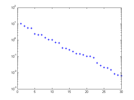
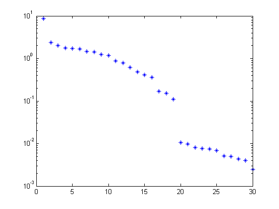
% parameters
n = 19;   % order of system
f = 30;   % future window size
p = 30;   % past window size

% PBSID-varx (open loop)
[S,X] = dordvarx(r,y,f,p,'tikh','gcv');
figure, semilogy(S,'*');
x = dmodx(X,n);
[Ai,Bi,Ci,Di,Ki] = dx2abcdk(x,r,y,f,p);

% PBSID-varmax (open loop)
[S,X] = dordvarmax(r,y,f,p,'els',1e-4,'tikh','gcv');
figure, semilogy(S,'*');
x = dmodx(X,n);
[Av,Bv,Cv,Dv,Kv] = dx2abcdk(x,r,y,f,p);
Verification results
% verification using variance accounted for (VAF) (open loop)
OLi = ss(Ai,Bi,Ci,Di,Ts);
OLv = ss(Av,Bv,Cv,Dv,Ts);
yr = lsim(OL(1,1),r,t);
yi = lsim(OLi,r,t);
yv = lsim(OLv,r,t);
disp('VAF with PBSIDopt-varx (high order)')
vaf(yr,yi)
disp('VAF with PBSIDopt-varmax (high order)')
vaf(yr,yv)
VAF with PBSIDopt-varx (high order)

ans =

   99.4845

VAF with PBSIDopt-varmax (high order)

ans =

   99.9933
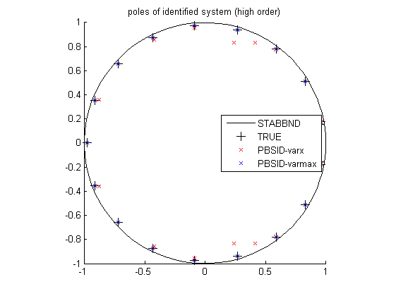
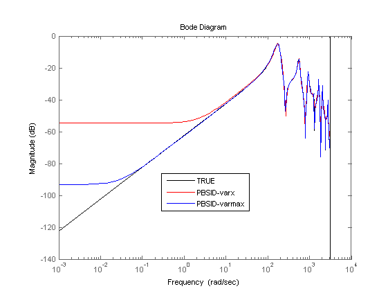
Identification results
% plot eigenvalues (high order)
figure
hold on
title('poles of identified system (high order)')
[cx,cy] = pol2cart(linspace(0,2*pi),ones(1,100));
plot(cx,cy,'k');
plot(real(pole(OL)),imag(pole(OL)),'k+','LineWidth',0.1,'MarkerEdgeColor','k','MarkerFaceColor','k','MarkerSize',10);
plot(real(eig(Ai)),imag(eig(Ai)),'rx');
plot(real(eig(Av)),imag(eig(Av)),'bx');
axis([-1 1 -1 1]);
axis square
legend('STABBND','TRUE','PBSID-varx','PBSID-varmax','Location','East');
hold off

% simulation
figure, bodemag(OL(1,1),'k',OLi,'r',OLv,'b');
legend('TRUE','PBSID-varx','PBSID-varmax','Location','Best');
Lower-order identification experiment
Identification of the model in open loop
% parameters
n = 9;    % order of system
f = 30;   % future window size
p = 30;   % past window size

% PBSID-varx (lower order)
[S,X] = dordvarx(r,y,f,p,'tikh','gcv');
x = dmodx(X,n);
[Ai,Bi,Ci,Di,Ki] = dx2abcdk(x,r,y,f,p);

% PBSID-varmax (lower order)
[S,X] = dordvarmax(r,y,f,p,'els',1e-4,'tikh','gcv');
x = dmodx(X,n);
[Av,Bv,Cv,Dv,Kv] = dx2abcdk(x,r,y,f,p);
Verification results
% verification using variance accounted for (VAF) (lower order)
OLi = ss(Ai,Bi,Ci,Di,Ts);
OLv = ss(Av,Bv,Cv,Dv,Ts);
yr = lsim(OL(1,1),r,t);
yi = lsim(OLi,r,t);
yv = lsim(OLv,r,t);
disp('VAF with PBSIDopt-varx (lower order)')
vaf(yr,yi)
disp('VAF with PBSIDopt-varmax (lower order)')
vaf(yr,yv)
VAF with PBSIDopt-varx (lower order)

ans =

   97.2436

VAF with PBSIDopt-varmax (lower order)

ans =

   50.7671
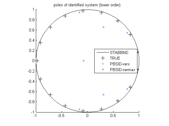
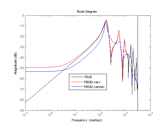
Identification results
% plot eigenvalues (lower order)
figure
hold on
title('poles of identified system (lower order)')
[cx,cy] = pol2cart(linspace(0,2*pi),ones(1,100));
plot(cx,cy,'k');
plot(real(pole(OL)),imag(pole(OL)),'k+','LineWidth',0.1,'MarkerEdgeColor','k','MarkerFaceColor','k','MarkerSize',10);
plot(real(eig(Ai)),imag(eig(Ai)),'rx');
plot(real(eig(Av)),imag(eig(Av)),'bx');
axis([-1 1 -1 1]);
axis square
legend('STABBND','TRUE','PBSID-varx','PBSID-varmax','Location','East');
hold off

% simulation
figure, bodemag(OL(1,1),'k',OLi,'r',OLv,'b');
legend('TRUE','PBSID-varx','PBSID-varmax','Location','Best');