Contents

Example 11: Slow-varying LTV model in open loop

close all; clear; clc;

The third-order LTV model with process noise

% Initial state-space of time-varying system
A0 = [0.8 -0.4 0.2; 0 0.3 -0.5; 0 0 0.5];
B0 = [0 0; 0 -0.6; 0.5 0];
C0 = [0.5 0.5 0; 0 0 1];
F0 = [0.055; 0.04; 0.045];
D0 = zeros(2);
G0 = [0.025; 0.03];

Open-loop identification experiment

Simulation of the model in open loop

% Simulation parameters
Ts = 1;
Tp = 2500;

% Simulation of time-varying system
t = 0:Ts:Tp; % time signal
u = randn(2,Tp+1); % input signal
w = 0.1.*randn(3,Tp+1); % noise signals
v = 0.1.*randn(2,Tp+1); % noise signals
x = zeros(3,1);
y = zeros(2,Tp+1);
E = zeros(3,Tp+1);
for i = 1:Tp+1
    if (i <= 665)
        A = A0;
    elseif (i > 665) && (i <= 2065)
        A(1,1) = A0(1,1) - 0.3*(exp(-(t(i)-665)/2000)-1)/(exp(-1)-1);
        A(2,2) = A0(2,2) - 0.5*(exp(-(t(i)-665)/2000)-1)/(exp(-1)-1);
        A(3,3) = A0(3,3) + 0.2*(exp(-(t(i)-665)/2000)-1)/(exp(-1)-1);
    end
    if (i <= 200)
        y(:,i) = C0*x + D0*u(:,i) + 0.001.*G0.*w(i);
        x = A*x + B0*u(:,i) + 0.001.*F0.*v(i);
    else
        y(:,i) = C0*x + D0*u(:,i) + G0.*w(i);
        x = A*x + B0*u(:,i) + F0.*v(i);
    end
    E(:,i) = eig(A);
end

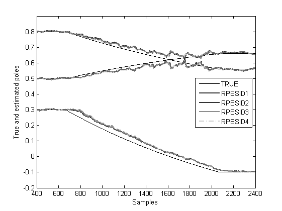
Identification of the model in open loop

% Recursive Subspace Identification parameters
n = 3;          % number of states
p = n + 2;      % past window size
f = n;          % past window size
lambda = 0.98;  % forgetting factor
ireg = 1e-6;     % initial regularisation
rlsopts = struct('ireg',[ireg ireg ireg],'lambda',[lambda lambda lambda],'reg',0);

% Start Recursive Subspace Identification
idopts = struct('method','varx','weight',1,'ltv',0,'noD',0,'past',0,'Kalm',0);
[Ak,Bk,Ck,Dk,Kk,err1,eigA1,dampA1] = rpbsid(u,y,f,p,n,[],idopts,rlsopts);

idopts = struct('method','varx','weight',1,'ltv',0,'noD',0,'past',1,'Kalm',0);
[Ak,Bk,Ck,Dk,Kk,err2,eigA2,dampA2] = rpbsid(u,y,f,p,n,[],idopts,rlsopts);

idopts = struct('method','varx','weight',1,'ltv',1,'noD',0,'past',0,'Kalm',0);
[Ak,Bk,Ck,Dk,Kk,err3,eigA3,dampA3] = rpbsid(u,y,f,p,n,[],idopts,rlsopts);

idopts = struct('method','varx','weight',1,'ltv',1,'noD',0,'past',1,'Kalm',0);
[Ak,Bk,Ck,Dk,Kk,err4,eigA4,dampA4] = rpbsid(u,y,f,p,n,[],idopts,rlsopts);

% Plot eigenvalues over time
figure,
t = 400:2400;
ELines  = plot(t,E(:,t),'k'); hold on
E1Lines = plot(t,real(eigA1(:,t)),'-.','LineWidth',1.5,'Color',[0.8 0.8 0.8]);
E2Lines = plot(t,real(eigA2(:,t)),'--','LineWidth',1.5,'Color',[0.6 0.6 0.6]);
E3Lines = plot(t,real(eigA3(:,t)),'-.','LineWidth',1.5,'Color',[0.4 0.4 0.4]);
E4Lines = plot(t,real(eigA4(:,t)),'-','LineWidth',1.5,'Color',[0.2 0.2 0.2]);
EGroup  = hggroup;
E1Group = hggroup;
E2Group = hggroup;
E3Group = hggroup;
E4Group = hggroup;
set(ELines,'Parent',EGroup)
set(E1Lines,'Parent',E1Group)
set(E2Lines,'Parent',E2Group)
set(E3Lines,'Parent',E3Group)
set(E3Lines,'Parent',E4Group)
set(get(get(EGroup,'Annotation'),'LegendInformation'),'IconDisplayStyle','on'); % Include this hggroup in the legend
set(get(get(E1Group,'Annotation'),'LegendInformation'),'IconDisplayStyle','on'); % Include this hggroup in the legend
set(get(get(E2Group,'Annotation'),'LegendInformation'),'IconDisplayStyle','on'); % Include this hggroup in the legend
set(get(get(E3Group,'Annotation'),'LegendInformation'),'IconDisplayStyle','on'); % Include this hggroup in the legend
set(get(get(E4Group,'Annotation'),'LegendInformation'),'IconDisplayStyle','on'); % Include this hggroup in the legend
legend('TRUE','RPBSID1','RPBSID2','RPBSID3','RPBSID4','Location','East');
axis([400 2400 -0.2 0.9])
xlabel('Samples')
ylabel('True and estimated poles')

Published with MATLAB® 7.11