Contents

Example 19b: Stabilizing the predictor form of an identified LPV model

Using the LPV system of example 19, we demonstate a feature of lx2abcdk: this function can stabilze the predictor form of the identified model in a convex polytope around the scheduling data used in the identification. It does this by solving a minimization problem with LMI constraints. Without this stabilization, the predictor form may get unstable. This usually occurs when we use short data sequences for identification, and low noise levels so that the noise part of the model is not excited sufficiently. Install YALMIP and an SDP solver such as SEDUMI to use this feature.

close all; clear; clc;

Flapping dynamics of a wind turbine

% System matrices
A1 = [0 0.0734; -6.5229 -0.4997];
A2 = [-0.0021 0; -0.0138 0.5196];
A12 = [A1 A2];
B12 = [-0.7221 0; -9.6277 0];
C12 = [1 0 0 0];
D12 = [0 0];
n = size(A12,1);    % The order of the system
m = size(A12,2)/n;  % The number of scheduling parameters
r = size(B12,2)/m;  % The number of inputs
l = size(C12,1);    % The number of outputs

% make affine LPV system
M = idafflpv(A12,B12,C12,D12,eye(2),zeros(2,1),1);

LPV Bode diagram

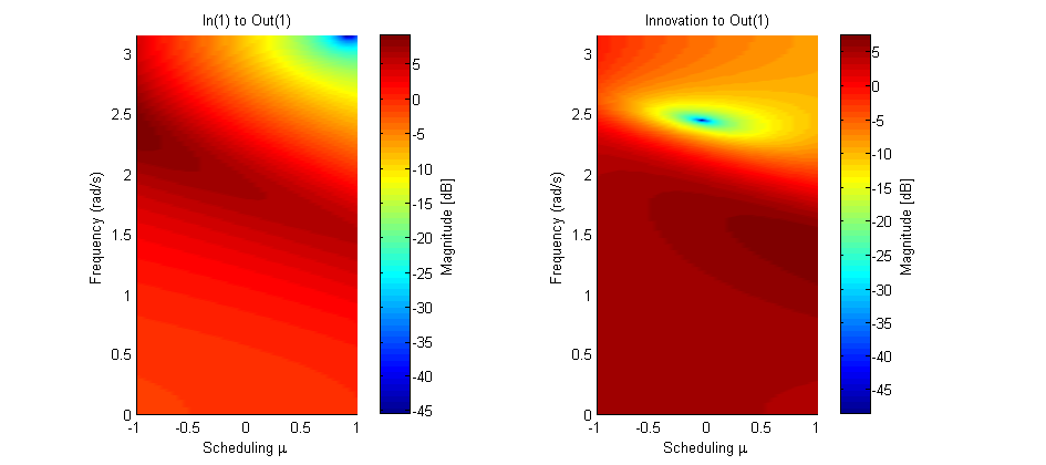
The PBSID toolbox Version 0.5 and higher includes a function bodemag for LPV models in the idafflpv object, displaying the varying Bode magnitude plots of the system.

h = bodemag(M,(-1:0.05:1)',0:0.01:pi,'colors');
set(h,'units','normalized','outerposition',[0.1 0.25 0.75 0.5])

Open-loop identification experiment

Simulation of the model in open loop, to obtain the data used in the identification experiment:

% defining a number of constants
j = 5;    % period
np = 10;  % number of periods
N = np*j;  % number of data points

% measured data from the scheduling parameters
mu3 = cos(2*pi*(1:N)'./j);

% simulation of the system with noise
t = (0:N-1)';
u = randn(N,r);
e = 0.01.*randn(N,l);
y0 = sim(M,u,t,mu3);
y = sim(M,u,t,mu3,e);
disp('Signal to noise ratio (SNR) (open-loop)')
snr(y,y0)

Signal to noise ratio (SNR) (open-loop)

ans =

   39.8172

Identification of the model in open loop

We generate system matrices A, B, C, D, K with lxabcdk. In Mkstable, the observer gain K is chosen such that the predictor form is stable.

% parameters
p = 5;     % past window size
f = 3;     % future window size

% LPV identification with noise
mu1 = ones(N,1);
mu = [mu1 mu3];
[S,x] = lordvarx(u,y,mu,f,p,'tikh','gcv',[0 1 0]);
x = lmodx(x,n);
[A,B,C,D,K] = lx2abcdk(x,u,y,mu,f,p,[0 1 0]);
Mk = idafflpv(A,B,C,D,K,zeros(2,1),1);

% Generating a predictor form that is guaranteed to be stable in a convex
% polytope around the scheduling data
[As,Bs,Cs,Ds,Ks] = lx2abcdk(x,u,y,mu,f,p,[0 1 0],0,1);
Mkstable = idafflpv(As,Bs,Cs,Ds,Ks,zeros(2,1),1);

Verification results

Simulation of identified LPV system:

yidk = sim(Mk,u,t,mu3,e);
disp('VAF of identified LPV system ')
vaf(y,yidk)

VAF of identified LPV system 

ans =

   97.4023

Simulation of identified LPV system in the predictor form. If the predictor form is not stable we get bad results.

x0 = findstates(Mk,u,y,t,mu3,'K');
yidpk = predict(Mk,u,y,t,mu3,x0,'K');
disp('VAF of predictions of identified LPV system (not guaranteed to be stable)')
vaf(y,yidpk)
x0 = findstates(Mkstable,u,y,t,mu3,'K');
yidpk = predict(Mkstable,u,y,t,mu3,x0,'K');
disp('VAF of predictions of stabilized predictor')
vaf(y,yidpk)

VAF of predictions of identified LPV system (not guaranteed to be stable)

ans =

     0

VAF of predictions of stabilized predictor

ans =

   97.0940

Stability analysis of the predictor form.

The function predstab returns the spectral radius at the cornerpoints of the convex polytope around the scheduling, and tau, the factor by which we can enlarge the scheduling range so that the predictor is still stable.

For non-stabilized predictor:

tau = predstab(Mk,min(mu3),max(mu3),'K',1,1)

cornerpoint:     mu = -0.81
spectral radius A-KC: 1.3
cornerpoint:     mu = 1
spectral radius A-KC: 1.1
cornerpoint:     mu = -0.81
spectral radius A-KC: 1.3
cornerpoint:     mu = 1
spectral radius A-KC: 1.1
Unable to stabilize for very small tau

tau =

  7.4506e-009

For stabilized predictor:

tau = predstab(Mkstable,min(mu3),max(mu3),'K',1,1)

cornerpoint:     mu = -0.81
spectral radius A-KC: 0.42
cornerpoint:     mu = 1
spectral radius A-KC: 0.34
cornerpoint:     mu = -0.81
spectral radius A-KC: 0.42
cornerpoint:     mu = 1
spectral radius A-KC: 0.34

tau =

    1.4715

Published with MATLAB® 7.11