Contents

Example 20: Fourth-order MIMO LPV model

close all; clear; clc;

Fourth-order MIMO Model

n = 4;  % The order of the system
m = 4;  % The number of scheduling parameters
r = 2;  % The number of inputs
l = 3;  % The number of outputs

% System matrices
A1 = [-1.3 -0.6325 -0.1115 0.0596; 1 0 0 0; 0 1 0 0; 0 0 1 0];
A2 = [-0.51 -0.1075 -0.007275 -0.0000625; 1 0 0 0; 0 1 0 0; 0 0 1 0];
A3 = [0.2 0 0 0; 0 0.4 0 0; 0 0 0 0; 0 0 0 0];
A4 = [0 0 0 0; 0 0 0 0; 0 0 0.3 0; 0 0 0 0.3];
B1 = [0 1; 1 0; 1 0; 0 1];
B2 = [0 0; 0 0; 0 0; 0.3 0.3];
B3 = B2;
B4 = B2;
K = [0.16 0 0; 0 0.16 0; 0 0 0.16; 0.16 0 0];
C = [1 0 0 0; 0 1 0 0; 0 0 1 0];
D = [0 0; 0 0; 0 0];
Alpv = [A1 A2 A3 A4];
Blpv = [B1 B2 B3 B4];
Clpv = [C zeros(l,3*n)];
Dlpv = [D zeros(l,3*r)];
Klpv = [K zeros(n,3*l)];

Open-loop identification experiment

Simulation of the model in open loop

% Measured data from the scheduling parameters
N = 1000;  % number of data points
t = (0:1:(N-1))';
rho = rand(N,1);
mu = [ones(N,1) rho 0.5.*sin((2*pi/100).*t).*rho 0.5.*cos((2*pi/100).*t).*rho];

% Measured input data
nu = randn(N,1);
eta = randn(N,1);
xi = randn(N,1);
[b,a] = butter(2,0.2);
u = [filter([0.75 1.05 0.15],1,eta) + filter(b,a,nu) xi];

% Simulation of the system without noise
M = idafflpv(Alpv,Blpv,Clpv,Dlpv,Klpv,[],1);
y0 = sim(M,u,t,mu(:,2:end));

% Simulation of the system with noise
e = 0.5.*randn(N,l);
y = sim(M,u,t,mu(:,2:end),e);
disp('Signal to noise ratio (SNR) (open-loop)')
snr(y,y0)

Signal to noise ratio (SNR) (open-loop)

ans =

   19.2396   19.2329   19.2336

Identification of the model in open loop

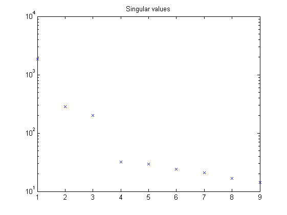
% Defining a number of constants
p = 5;     % past window size
f = 3;     % future window size

% LPV identification
[S,x] = lordvarx(u,y,mu,f,p,'tikh','gcv',[0 0 0]);
x = lmodx(x,n);
[Aid,Bid,Cid,Did,Kid] = lx2abcdk(x,u,y,mu,f,p,[0 0 0]);
[Aid1,Bid1,Cid1,Did1,Kid1] = lx2abcdk(x,u,y,mu,f,p,[0 0 0],1);
figure, semilogy(S,'x');
title('Singular values')

Optimization with the prediction error method

Mi = idafflpv(Aid,Bid,Cid,Did,Kid,[],1);
[e,x0] = pe(Mi,u,y,t,mu(:,2:end),'CD');
Mi.x0 = x0;
Mi.NoiseVariance = cov(e);
Mp = pem(Mi,u,y,t,mu(:,2:end),'CD');

maximum number of iterations has been exceeded

Validation results

% Validation data from the scheduling parameters
rho = rand(N,1);
mu = [ones(N,1) rho 0.5.*sin((2*pi/100).*t).*rho 0.5.*cos((2*pi/100).*t).*rho];

% Validation data
nu = randn(N,1);
eta = randn(N,1);
xi = randn(N,1);
[b,a] = butter(2,0.2);
u = [filter([0.75 1.05 0.15],1,eta) + filter(b,a,nu) xi];

% Simulation of the system without noise
y0 = sim(M,u,t,mu(:,2:end));

% Simulation of identified LPV system
yid = sim(Mi,u,t,mu(:,2:end));
disp('VAF of identified LPV system')
vaf(y0,yid)

% Simulation of optimized LPV system
yid = sim(Mp,u,t,mu(:,2:end));
disp('VAF of optimized LPV system')
vaf(y0,yid)

VAF of identified LPV system

ans =

   99.1401
   99.1739
   99.1748

VAF of optimized LPV system

ans =

   99.9826
   99.9827
   99.9824

Published with MATLAB® 7.9