Contents

Example 21: Second-order Periodic-LPV model of flapping dynamics

close all; clear; clc;

Flapping dynamics of a wind turbine

% System matrices
A1 = [0 0.0734; -6.5229 -0.4997];
A2 = [-0.0021 0; -0.0138 0.5196];
A12 = [A1 A2];
B12 = [-0.7221 0; -9.6277 0];
C12 = [1 0 0 0];
D12 = [0 0];
n = size(A12,1);    % The order of the system
m = size(A12,2)/n;  % The number of scheduling parameters
r = size(B12,2)/m;  % The number of inputs
l = size(C12,1);    % The number of outputs

Open-loop identification experiment

Simulation of the model in open loop

% Defining a number of constants
j = 10;     % period
np = 500;   % number of periods
N = np*j;   % number of data points

% measured data from the scheduling parameters
mu3 = cos(2*pi*(1:N)'./j) + 0.2;

% make affine LPV system
M = idafflpv(A12,B12,C12,D12,eye(2),zeros(2,1),1);

% simulation of the system with noise
t = (0:N-1)';
u = randn(N,r);
e = 0.1.*randn(N,l);
y0 = sim(M,u,t,mu3);
y = sim(M,u,t,mu3,e);
disp('Signal to noise ratio (SNR) (open-loop)')
snr(y,y0)

Signal to noise ratio (SNR) (open-loop)

ans =

   18.6035

Identification of the model in open loop

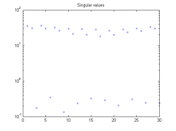
% parameters
p = 5;     % past window size
f = 3;     % future window size

% LPV identification with noise
mu1 = ones(N,1);
mu = [mu1 mu3];
pnd = pschedclust(mu,f,p);
[S,x,TU,K] = pordvarx(u,y,mu,f,p,pnd,'tikh','gcv',0,[0 0 1 1 0]);
[x,CC] = pmodx(x,TU,K,n,1e-4,1e-8);
[A,B,C,D,K] = px2abcdk(x,u,y,mu,f,p,[0 0 1 1 0],pnd);
figure, semilogy(S(:),'x');
title('Singular values')
disp('Canonical correlation coefficients (no noise)')
CC(1:n)

Canonical correlation coefficients (no noise)

ans =

    1.0000    1.0000

Verification results

% Simulation of identified LPV system
Mk = idafflpv(A,B,C,D,K,zeros(2,1),1);
yidk = sim(Mk,u,t,mu3,e);
disp('VAF of identified LPV system ')
vaf(y,yidk)

VAF of identified LPV system 

ans =

   97.3130

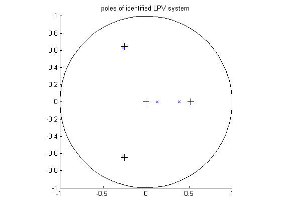
Identification results

% Plot eigenvalues
figure
hold on
title('poles of identified LPV system')
[cx,cy] = pol2cart(linspace(0,2*pi),ones(1,100));
plot(cx,cy,'k');
plot(real(eig(A1)),imag(eig(A1)),'k+','LineWidth',0.1,'MarkerEdgeColor','k', 'MarkerFaceColor','k', 'MarkerSize',10);
plot(real(eig(A(1:n,1:n))),imag(eig(A(1:n,1:n))),'bx');
plot(real(eig(A2)),imag(eig(A2)),'k+','LineWidth',0.1,'MarkerEdgeColor','k', 'MarkerFaceColor','k', 'MarkerSize',10);
plot(real(eig(A(1:n,n+1:2*n))),imag(eig(A(1:n,n+1:2*n))),'bx');
axis([-1 1 -1 1]);
axis square
hold off

Published with MATLAB® 7.9