Contents
Getting Started
The LTI System Identification Toolbox for Matlab enables you to perform an identification of linear time-invariant systems. It provides command-line functions for parametric model estimation and subspace model identification in both discrete-time and continuous-time (frequency domain). To get you started, this page will explain a subspace identification of a small LTI model using the PI-MOESP method. For more examples and a full description of the functions, read the toolbox software manual.
Subspace Identification using PI-MOESP
In this example we will give an example of how the subspace identification framework in the toolbox software is used in a practical situation. The PI-MOESP scheme functions dordpi and dmodpi will be used to estimate A and C, after which dac2bd and dinit are used to estimate B, D and the initial state. Finally, a simple model validation is performed.
First we generate data for a second-order system. Apseudorandom binary sequence will be generated as identification input using the tool prbn. A pseudo-random binary sequence, or PRBN, is an often-used identification input signal. In the following example, the rate is set to 0.1 in order to get a signal that changes state rather infrequently and which therefore mainly contains signal energy in the lower frequency range.
A = [1.5 -0.7; 1 0]; B = [1; 0]; C = [1 0.5]; D = 0;
u = prbn(300,0.1)-0.5;
y = dltisim(A,B,C,D,u);
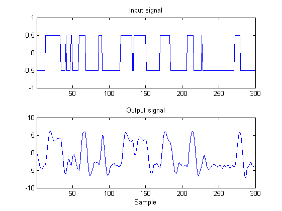
In order to make the example more realistic, the output signal is disturbed by colored measurement noise such that a 20 dB SNR is obtained. The b and a vectors correspond to the numerator and denominator polynomials of a lowpass filter.
b = [0.17 0.50 0.50 0.17];
a = [1.0 0 0.33 0];
y = y + 0.1*std(y)*filter(b,a,randn(300,1));

figure, subplot(2,1,1);
plot(1:300,u);
title('Input signal')
axis([1 300 -1 1]);
subplot(2,1,2);
plot(1:300,y);
title('Output signal')
axis([1 300 -10 10]);
xlabel('Sample')
We will now try to identify the system from the generated data set by assuming the following state-space model structure:


This model, in which v(k) is a colored noise signal, falls within the class of models for which PI-MOESP can provide consistent estimates, as was illustrated in Section 9.5 of the textbook.
Step 1: Data Compression and Order Estimation
In this first step we use the "ord" function, dordpi in this PI-MOESP case, in order to compress the available data and to generate a model order estimate. The only model structure selection parameter that we need to pass is the block-size s, which should be larger than the expected system order. We will use the rather high value s=10 in this example in order to show the order selection mechanism more clearly.
s = 10;
[S,R] = dordpi(u,y,s);
The function dordpi returns a vector S containing singular values based on which the model order can be determined. In addition, a compressed data matrix R is returned that is used by dmodpi to estimate A and C in the next step. The singular values in S are plotted using the following command:
figure, semilogy(1:10,S,'x')
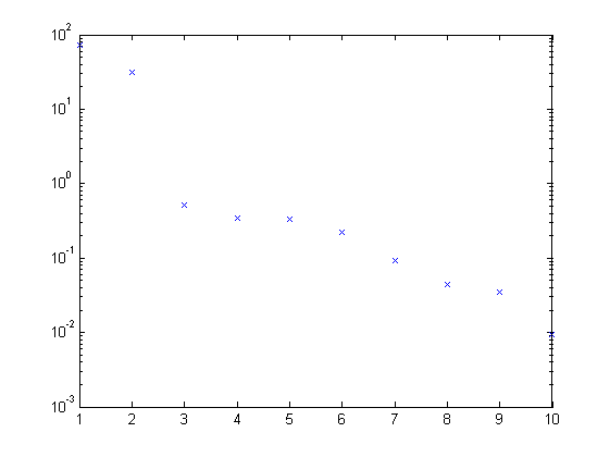
In a noise-free case, only the first n singular values would have been nonzero. However, the singular values that would have been zero are now disturbed because of the noise. Still, a gap is visible between singular values 2 and 3, and so the model order will be chosen equal to n=2.
Step 2: Estimation of A and C
In this step we will obtain estimates for A and C. As the A and C variables have already been defined, we will call the estimates for A and C, Ae and Ce respectively. The function dordpi is used to determine Ae and Ce based on the R matrix from dordpi and the model order n determined from the singular value plot.
n = 2;
[Ae,Ce] = dmodpi(R,n);
Step 3: Estimation of B, D and the Initial State
Once estimates Ae and Ce for A and C have been determined, the toolbox function dac2bd will be used to estimate B and D, as Be and De respectively. The function dac2bd requires the estimates for A and C and the measured inputoutput data. Subsequently, the toolbox function dinit is used to obtain the initial state x0 corresponding to the current data set. This function needs estimates for all system matrices as well as the measured input-output data.
[Be,De] = dac2bd(Ae,Ce,u,y);
x0e = dinit(Ae,Be,Ce,De,u,y);
Model Validaton
The quality of the model (Ae,Be,Ce,De) that has been identified will now be assessed. To this end, we will compare the output predicted by the identified model to the measured output signal. As a figure of merit, we use the variance accounted for (VAF). If the model is good, the VAF should be close to 100%. The following code fragment simulated the estimated model using the measured input signal in order to obtain the estimated output ye. Subsequently, the VAF is calculated using the toolbox function vaf.
ye = dltisim(Ae,Be,Ce,De,u,x0e);
vaf(y,ye)
ans =

   99.4524
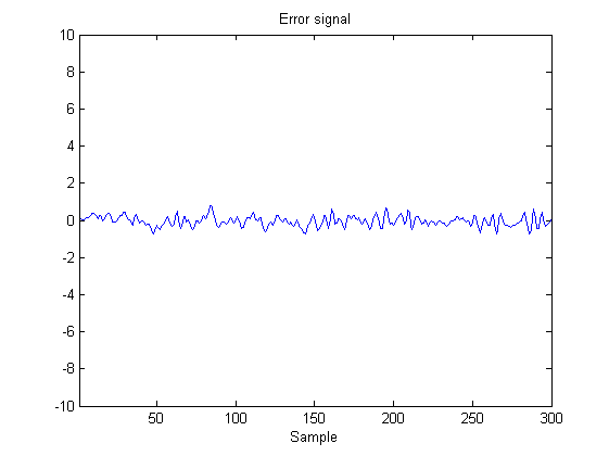
It is clear that the estimated model described the actual system behavior well. The error signal y(k) - ye(k) is plotted. This error is very small compared to the output signal in the first figure.
figure, plot(1:300,y-ye);
title('Error signal')
axis([1 300 -10 10]);
xlabel('Sample')